Association Test with Principal Components

Introduction

Latent variables (LVs) are unobserved and must be estimated directly from the data, using PCA and others. However, treating PCs as independent variables in a regression framework or a correlation test is circular analysis, producing anti-conservative biases and spurious associations. The jackstraw accounts for the fact that PCs are calculated from the data and to protect association tests from an anti-conservative bias.

R package installation

The jackstraw R package is used for the association test. A few other packages are necessary to run this tutorial.

# install or update these packages
# install.packages(c("jackstraw","corpcor","RColorBrewer"))

library(jackstraw) # for the jackstraw methods
library(corpcor) # for fast SVD
library(RColorBrewer) # for colors

Latent Variable Models

Latent variable models (LVM) are frequently used in data analysis explicitely or implicitely. Latent variables (LVs) can be seen as underlying sources of variation, that are hidden and/or undefined. In some cases, sources of variation may be directly measured, such as disease status or sex, and conventional association tests can be utilized to assess statistical significance of association between variables and such (independent and external) measurements. However, underlying sources of variation may be impossible to measure or poorly defined, such as cancer subtypes or population structure. For example, cancer subtypes based on histological tumor classification are highly imprecise. Therefore, it is a popular approach in genomics to estimate cancer subtypes using gene expression or other molecular data.

When we have a high-dimensional data where a large number of variables (e.g., genes) are measured for each sample, LVs are often estimated by PCA. After applying PCA to the observed data, one may like to identify variables associated with a set of PCs. To do this association testing while adjusting for over-fitting problem, we use the jackstraw test.

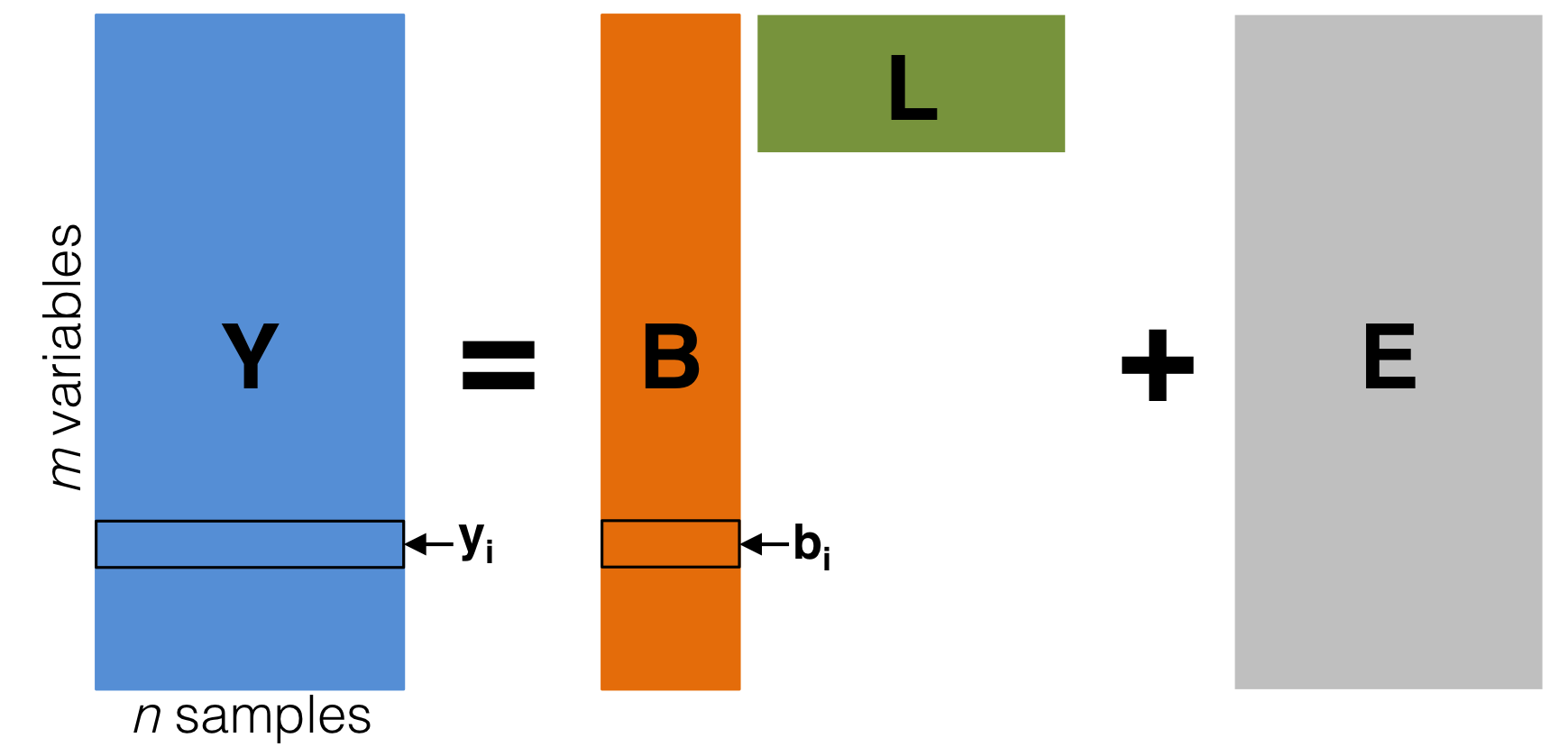
_{Diagram of the latent variable model \(\mathbf{Y} = \mathbf{BL} + \mathbf{E}\). The latent variable basis \(\mathbf{L}\) is not observable, but may be estimated from \(\mathbf{Y}\). The noise term \(\mathbf{E}\) is independent random variation. We are interested in performing statistical hypothesis tests on \(i\) (\(i=1, \ldots, m\)), which quantifies the relationship between \(\mathbf{L}\) and \(y_i\) (\(i=1, \ldots, m\)).}

Simulated Continous Data (e.g., Gene Expression)

We simulate a simple gene expression data with \(m=1000\) genes (or variables) and \(n=20\) samples (or observations). The following simulation code generates a dichonomous mean shift between the first set of 10 samples and the second set of 10 samples. This may represent a case-control study, where an external/environmental factor influneces samples differentially. This mean shift affects \(10\%\) of \(m=1000\) genes (as indicated by a color bar on rows):

library(jackstraw) # for the jackstraw methods
library(corpcor) # for fast SVD
library(RColorBrewer) # for colors

set.seed(1)
B = c(runif(100, min=0, max=1), rep(0,900))
L = c(rep(.5, 10), rep(-.5, 10))
L = L / sd(L)
E = matrix(rnorm(1000*20), nrow=1000)
Y = B %*% t(L) + E
Y = t(apply(Y, 1, function(x) scale(x,center=TRUE,scale=FALSE)))

coul <- colorRampPalette(brewer.pal(11, "RdBu"))(50)
heatmap(Y,Rowv=NA,Colv=NA, col = coul,
        RowSideColors=c(rep("black",100),rep("lightgrey",900)),
        ColSideColors=c(rep("blue",10),rep("red",10)))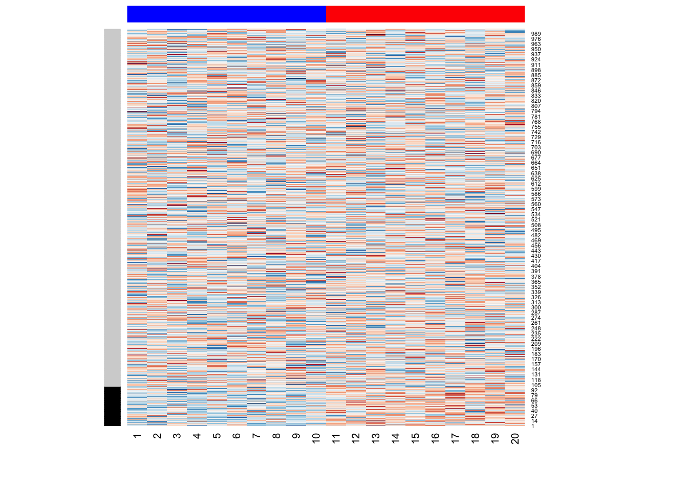

Please note that we know that there’s only \(r=1\) PC, because the data is simulated. In practice, one needs visual and statistical approaches to estimate \(r\). For a starter, we can visualize the variance explained with a scree plot. A simple permutation approach based on parallel analysis from Buja and Eyuboglu (1992)² is implemented as jackstraw::permutationPA function. Some of great statistical literature on determining the number of PCs/LVs include Anderson (1963), Tracy and Widom (1996), Johnstone (2001), and more³. For R implementations and heuristics, check out nFactors and PCDimension

# compute PCA via SVD (corpcor::fast.svd)
svd.out = corpcor::fast.svd(Y)

plot(svd.out$d^2/sum(svd.out$d^2), pch=20, main="The scree plot", xlab="PC", ylab="Percent Variance Explained")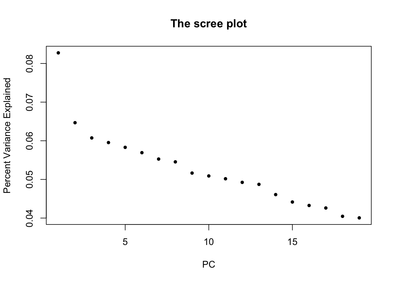

plot(svd.out$d[1] * svd.out$v[,1], pch=20, main="1st PC", xlab="Observation", ylab="Magnitude")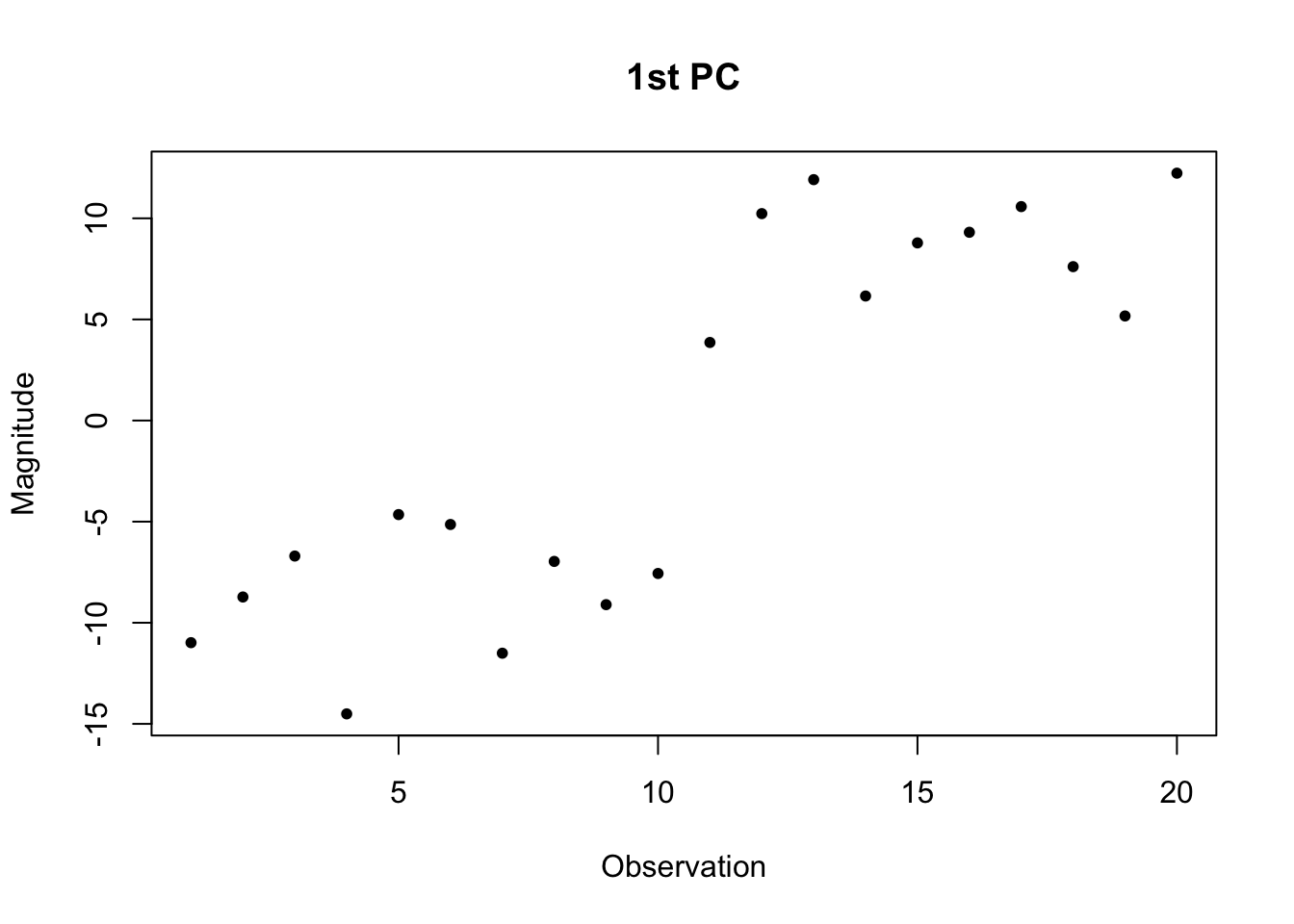

# optionally, run permutation parallel analysis.
# check out nFactors and PCDimension for more methods
PA = permutationPA(Y, B=10, threshold=0.05, verbose=FALSE)

The jackstraw test of association using principal components

We are now ready to apply the jackstraw to our data, in order to assess statistical significance of association between variables and the first PC:

js.pca = jackstraw_pca(Y, r = 1, s = 10, B = 1000, verbose = FALSE)

hist(js.pca$p.value, 20, col="black")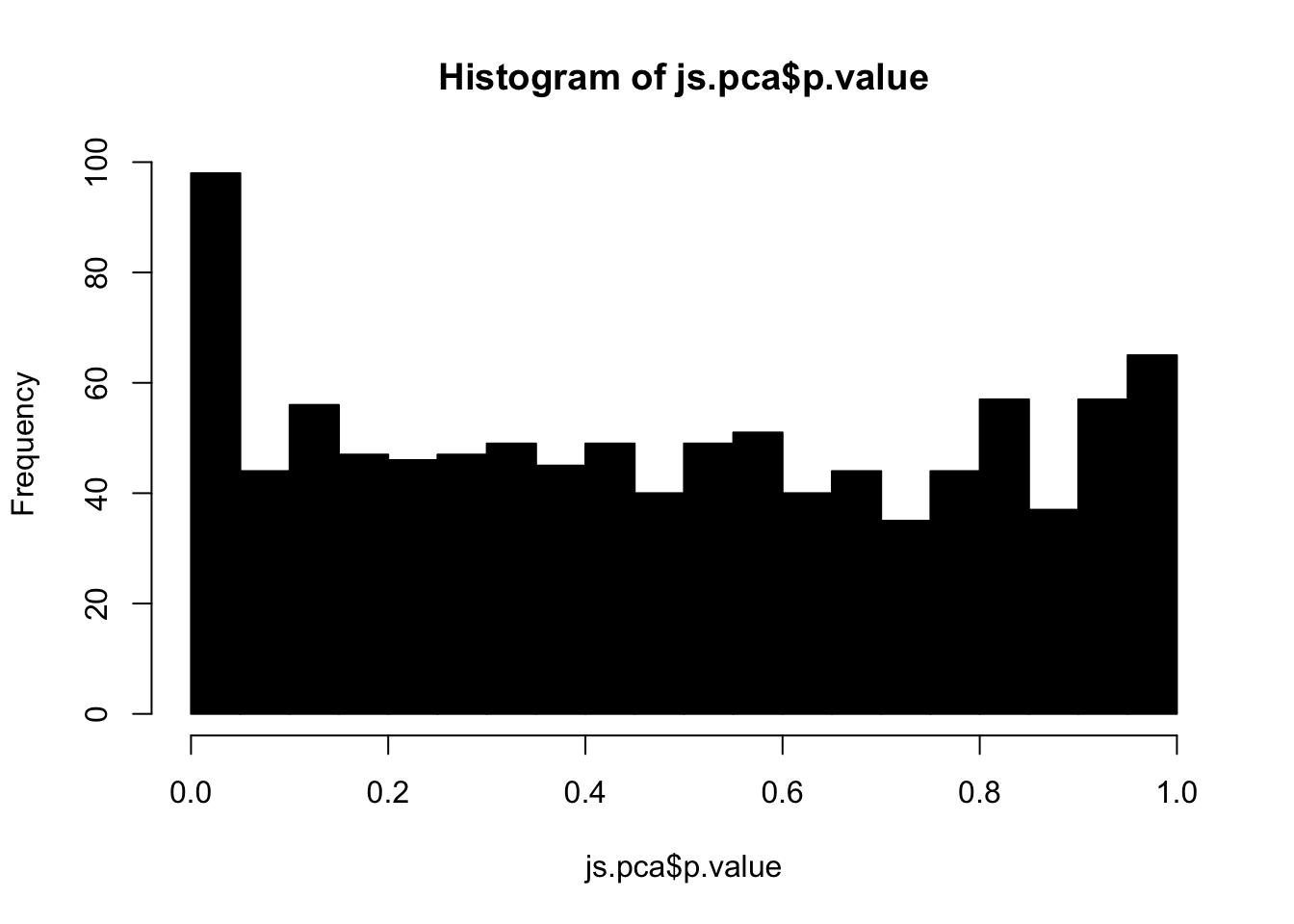

Since the data was simulated, we can visualize the p-values for null hypotheses (variables that do not exhibit true difference between two groups). We call these null p-values. Alternatively, alternative p-values are for alternative hypothesis (variables that do exhibit true difference between two groups). By definition, the set of null p-values should follow i.i.d. uniform distribution between 0 and 1:

par(mfrow=c(2,1))
hist(js.pca$p.value[1:100], 10, col="black", main="Alternative P-values")
hist(js.pca$p.value[101:1000], 10, col="black", main="Null P-values")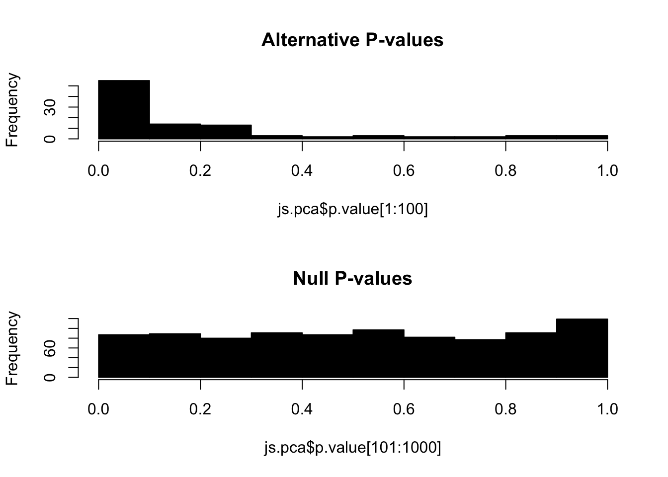

The jackstraw algorithm

We aim to estimate an empirical distribution of F-statistics statistics under the null hypothesis that a variable is not associated with a PC(s).

The jackstraw randomly chooses S variables (or rows in our example), where S is much smaller than N (N >> S). Each of S variables is permuted, resulting in S synthetic variables. The jackstraw data is a hybrid dataset consisted of N-S observed variables and S synthetic null variables. Then, PCA is applied on the jackstraw data, where F-statistics between S synthetic nulls and that PC are calculated. By repeating this resampling strategy B times, we obtain B * s null statistics, that forms an empirical distribution.

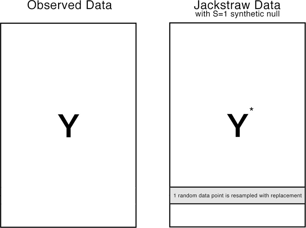
_{Diagram of the jackstraw data. In this example of S=1, one row is randomly chosen and independently permuted. Systematic variation in \(\mathbf{Y}\) and \(\mathbf{Y}^*\) are almost identical when S >> M, such that PCs are also preserved. Then, synthetic nulls can be used to calculate the empirical distribution of null F-statistics.}